What is Ansys Forming?

Ansys Forming is an end-to-end tool for sheet metal manufacturing process simulation; it has truly redefined how sheetmetal forming is being done using our trusted LS-DYNA solver. It has a newly developed graphical user interface that allows engineers to easily, accurately and efficiently setup the simulation, solve the job and analyze the results. The advantage of our Ansys Forming software is that most of the parameters are already predefined and user is interactively guided through a streamlined step by step process. Ansys Forming only needs the knowledge of the sheetmetal forming process. In a nutshell, Ansys Forming is a one stop shop for all metal stamping needs and it offers an optimal performance delivering a good balance between speed and accuracy.

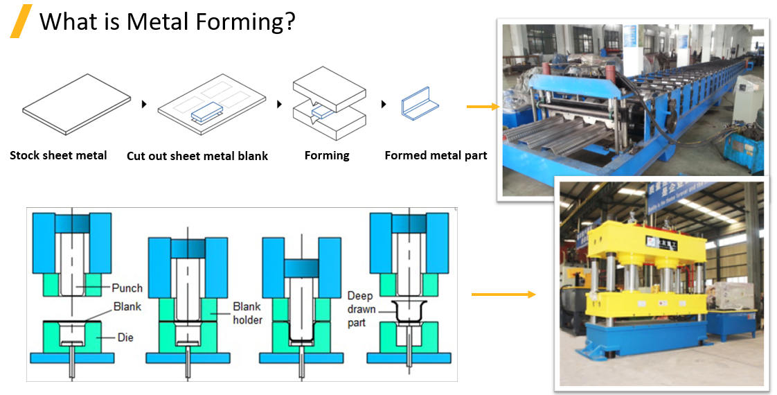
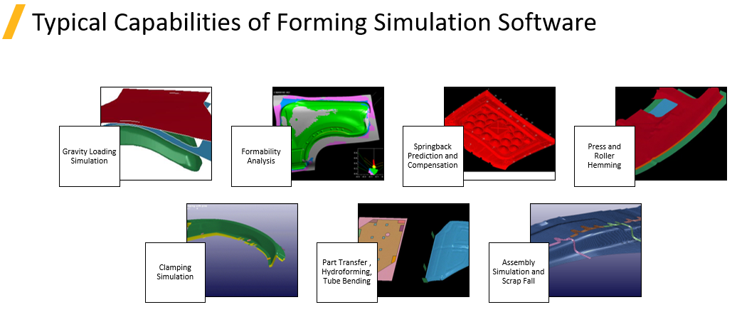
In Ansys Forming “Deep drawing” is the process we are trying to simulate. The forming process is typically performed on a press and the parts are formed between 2 dies as shown above. This is a time intensive process and the procedure requires machinery and specialized tools. Through Ansys Forming we are able to simulate gravity loading simulation, conduct formability analysis, account for springback prediction and compensation, conduct press and roller hemming, perform clamping simulation, account for hydroforming, etc. as shown on the graphic below. In Forming simulation, the desired shape is extracted through plastic deformation w/o undergoing any advanced machining processes such as milling. With Ansys Forming we can optimize the process before the actual tool is manufactured. It reduces the cost to manufacture the tools and reduces the time to market for OEM’s. It guarantees the manufacturability of the parts and ensures parts come out right the first time.

What are some common applications of Ansys Forming?

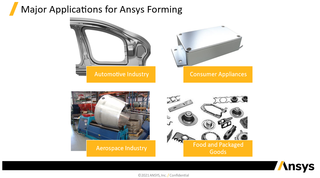
Most of the applications for Ansys Forming are found in the following industries ranging from Automotive OEMS, suppliers manufacturing fenders, doors, hoods and various parts and accessories of the automobile to Aerospace manufacturing various parts of the entire aircraft including wings, fuselage, etc. from Consumer appliances such as refrigerators and washing machines to food and packaging industry manufacturing cookware, canned products, etc. the application is quite widespread.

Join us on July 30, 2024, at 9:00 AM for our exclusive webinar and discover how Ansys Forming can revolutionize your sheet metal manufacturing process!

In an increasingly competitive landscape, companies invest heavily in reducing costs and time to market. Traditional techniques of modeling, testing, and prototyping are no longer viable. Using computer-aided engineering (CAE), companies can mimic physical drop tests and impact tests at a fraction of the cost, saving millions of dollars. With Ansys LS-DYNA, companies can simulate material failure, component deformation, and energy absorption related to various test standards and specs.When was the last time you had the harrowing experience of dropping your expensive smartphone on the road while loading your groceries into your car, ending up with a cracked screen? Or perhaps you damaged your smartwatch by hitting it against a doorknob? Consumer electronics are highly susceptible to damage from accidents and shipping mishaps, leading to costly replacements and customer dissatisfaction. Companies are constantly exploring innovative ways to improve product design for better sustainability and durability against impacts and drops.

The Widespread Application of Drop and Impact Testing

The application of drop testing extends beyond consumer electronics. It includes:

• Automotive Industry: Vehicle front-end collision with a concrete barrier.
• Aviation Industry: Bird strikes on the leading edge of an aircraft.
• Transportation Sector: Packages dropped during transit.
• Military Applications: Impact of kinetic energy projectiles like bullets piercing armor plates.

Using our Ansys LS-DYNA explicit simulation capabilities, users are able to simulate drop tests and impact tests much more comprehensively and efficiently.

What are the Advantages of Running Computer Aided Simulation?

In the ever increasing cutthroat competitive landscape companies are heavily invested in ways to reduce cost and time to market and the traditional technique of modeling, testing and prototyping is not a viable option anymore. Using computer-aided engineering (CAE) companies are able to mimic these physical drop tests and impact tests which are otherwise very expensive and time consuming at a fraction of the cost which can save companies millions of dollars. Using our Ansys LS-DYNA tool, companies are able to simulate drop tests to simulate material failure, component deformation, energy absorption related to various test standards and specs. With our tool creating a virtual prototype is fast and easy and facilitates easy design iteration process that yields fast and reliable results and the ROI on the software investment is more than justified when comparing this to expensive physical tests.

Drop Test and Impact Test Simulations with Ansys LS-DYNA

Cell Phone Drop Test

This simulation involves dropping a generic mobile phone from a height to impact with the ground.

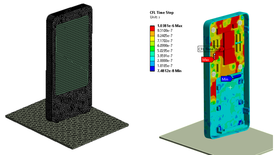
The mesh count was well under 30k elements and CFL timestep was plotted to ensure we could use small amount of mass scaling to expedite the solve if needed as shown below.

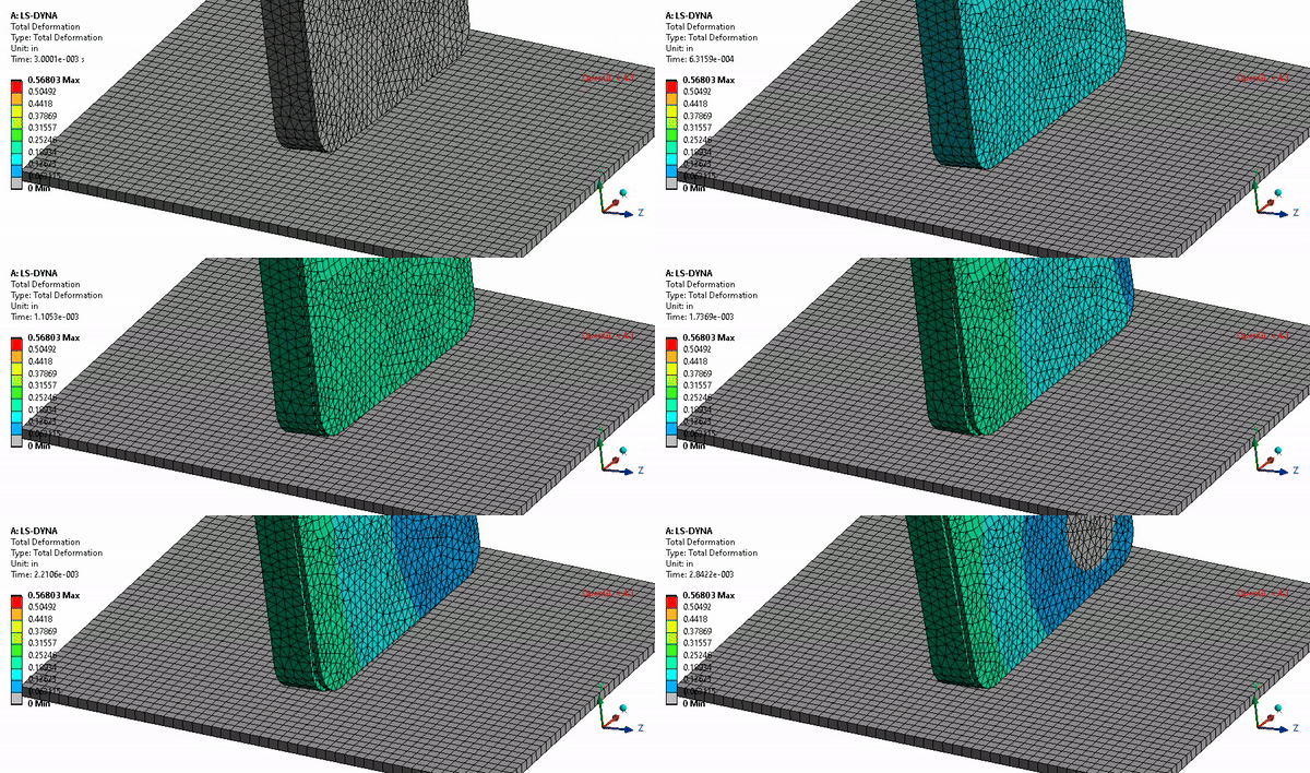
The animation below shows the result from the cell impacting the ground.

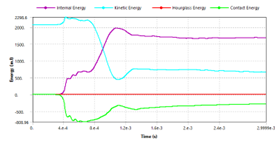
The animation above reveals the battery pack separating from the lower housing due to frictional sliding which attributes to the negative contact energy as observed on the plot below for energy summary.

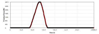
In addition to stresses and deformation on the various objects we can also gather useful information on contact force transmitted between the device and ground as shown below.

Bird strike on the leading edge of an aircraft 

Bird strikes are fairly common occurrence that can happen when the aircraft is flying at low altitudes especially in situations of take off and landing. The bird strikes can be quite catastrophic if the bird strikes the windshield of an aircraft or gets sucked into the engine or as in this case hits the leading edge of the airfoil of the aircraft that can cause structural damage.

The aviation industry is heavily focused on not only ensuring that such occurrences do not occur but in the circumstances, they do occur that the structural integrity of the aircraft is not compromised.

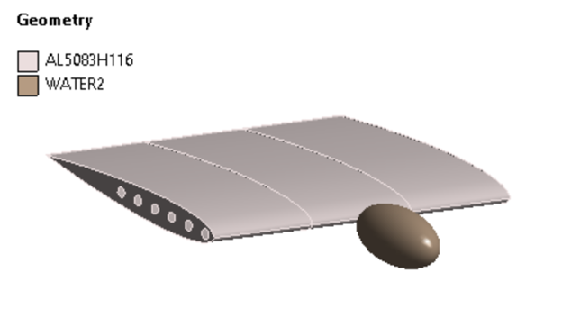
In this example the airfoil which is the structural part (“Lagrangian” body) is comprised of a Multibody part comprising of an outer skin and four interior stiffeners inside. The airfoil material is defined as “Aluminum” and is modeled in Ansys LS-DYNA using the Johnson Cook strength material model. The bird is idealized as an “ellipsoid” shape and simulated using Smooth Particle Hydrodynamics (SPH) in LS-DYNA. The material assigned to the bird is “water” which includes an equation of state and tensile pressure failure set to 0 Pa to easily allow the body of the bird to disintegrate on impact. The graphic below explains the various aspects of the geometry and material setup.

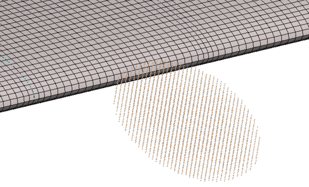
Provided below is a closeup view of the finite element mesh. The mesh reveals the airfoil which is the “Lagrangian” part and the bird is defined as “SPH” part viewed as particle mesh.

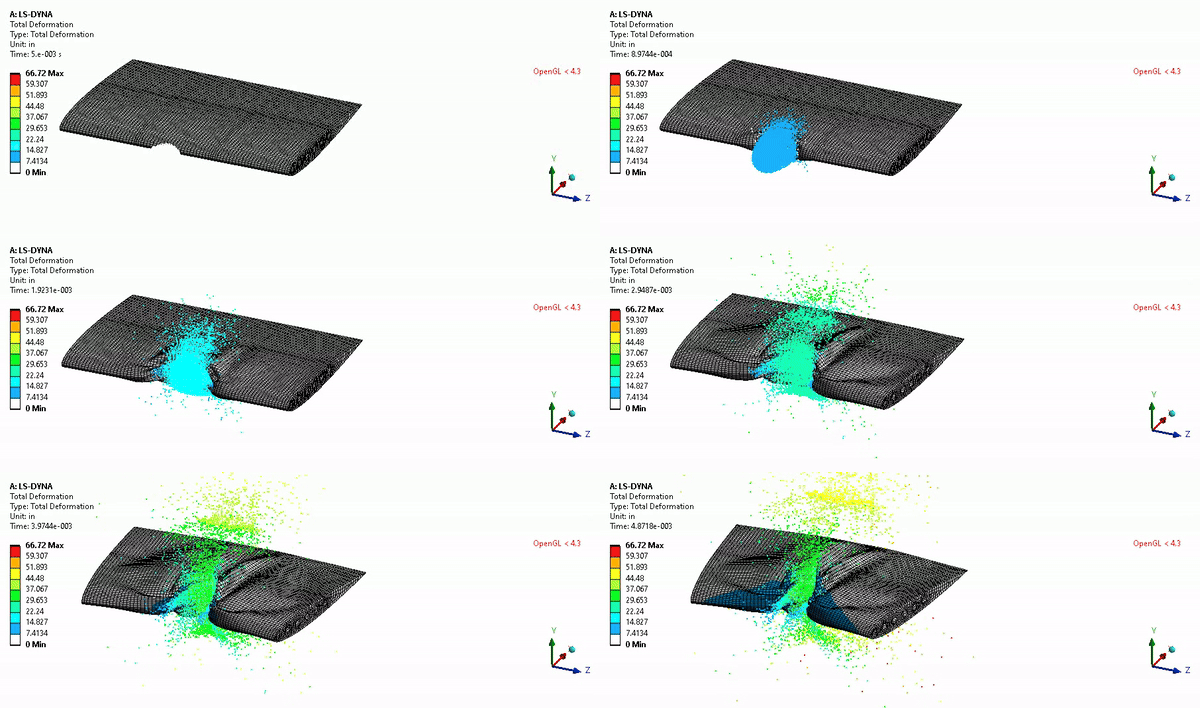
The bird is designed to impact the aircraft approaching at approximately 900 km/hr to mimic the speed of the aircraft at time of impact. Provided below are snapshots of the plastic strain and deformation showing extensive damage to the airfoil structure post impact.

Provided below is an animation of the bird strike simulation.

Maritime collision

The rapid increase in maritime traffic makes risk of collision higher in areas of high traffic places. The consequences of ship collision can be quite catastrophic which can be detrimental to not only the environment but also put the ships crew under risk and hence a huge amount of emphasis is put into consideration in the design stage of the ship.

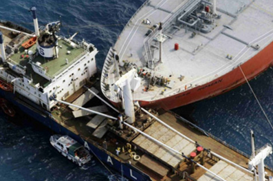
The graphic below shows the collision between a tanker and ferry and this impact simulation was solved using Ansys LS-DYNA.

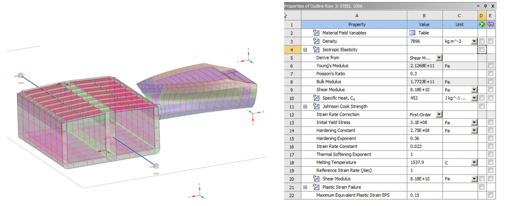
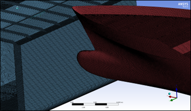
The tanker and ferry were defined as “Lagrangian” parts; Johnson Cook material model was used to define the elastic-plastic behavior and the plastic strain failure was used to simulate failure. The graphics below show the finite element mesh for the simplified model taken into consideration and material law used.

The initial velocity of 3 m/s was applied to the cruise ship and contact was defined as single surface contact to ensure self-impact.

Provided below are graphics of the plastic deformation showing significant damage on the hull of the fuel tanker.

The animation below captures the simulation of the collision between the tanker and ferry.

The applications above demonstrate the power behind virtual prototyping to simulate any sort of drop test or impact test and Ansys LS-DYNA is able to calibrate test results very closely.

Explore the Full Potential of Ansys LS-DYNA

The applications above demonstrate the power of virtual prototyping to simulate various drop and impact tests. Ansys LS-DYNA can calibrate test results very closely, offering significant advantages over traditional testing methods.

Don’t Miss Our Webinar on Advanced Simulation Techniques! Register now!

There are situations in which it may be necessary to tweak friction coefficient in a nonlinear contact analysis during the simulation. Currently, the Ansys Workbench GUI does not support this capability directly; however, it is possible to vary the friction coefficient using a command object.

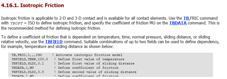
The Ansys documentation has several references of doing this as listed under the Help section; Mechanical APDL > Material Reference > Nonlinear Material Properties > Contact Friction as shown below.

This section on the documentation describes defining contact friction using TB,FRIC which is a material property used with current technology contact elements. It can be used to define coefficient of friction for both isotropic or orthotropic friction models. It further discusses varying friction coefficient in a multiple load step scenario, as well as implementing user defined friction  using TB,FRIC with TBOPT = USER.

The example presented here will show how to use commands object within Workbench to vary friction coefficient. The friction coefficient is defined via the TB,FRIC command. To define the friction that is function of temperature, time, normal pressure, sliding distance, etc. you can use the TBFIELD command in conjunction with the TB,FRIC. In this example presented, the friction is varied with time (to simulate it’s change through the load step).

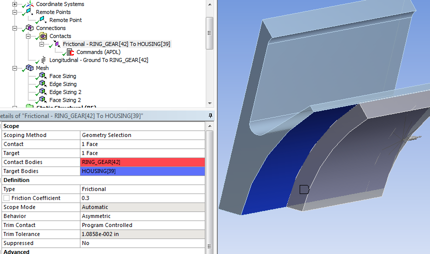
Below is a graphic of the nonlinear contact between the Aluminum housing and steel ring gear.

The command object used to modify friction as a function of time is shown below.

This command object uses the information in the table below to modify friction :

Time                Friction Coefficient
0                      0
0.2                  0.1
0.4                  0.3
0.6                  0
0.8                  0.15
1                      0

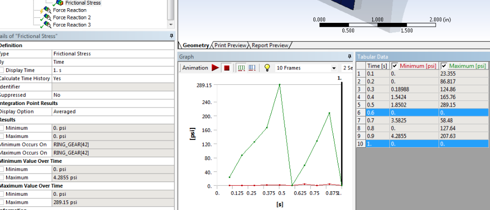
As an example of the friction can vary, notice the friction coefficient is zero for time = 0.6 and time = 1.0.

During the run, the output controls under Analysis Settings was set to Yes for Nodal Forces, Contact Miscellaneous and General Miscellaneous.

A quick look at the contact results confirms our findings. The contour plot for contact friction stress shows zero results for time = 0.6 and 1 which m

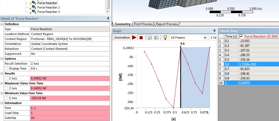
Another sanity check is to check for reaction force through the frictional contact with the extraction method set to contact element option; this also reveals zero (nearly zero reaction force at these time points). The very small discrepancy noted on the reaction force is due to a few overlapping nodes on a boundary condition.

Often there is a need to export the deformed geometry from Ansys Mechanical. Possibly to a 3D printer to show to customers, or maybe a new CAD geometry file is needed that can be used for drawings or further design evaluation. Ansys Mechanical offers two options for users for doing this task.

Exporting STL (Standard Tessellation Language) files from the deformed results is one option. The STL file may be opened within Ansys Discovery and reverse engineered to create deformed solid geometry from the STL facets.

I have posted a YouTube video that demonstrates this technique. In the video, I have a rubber cushion that is compressed between two metal plates as shown. The rubber geometry gets deformed and the goal here is to export the deformed faceted geometry and create smooth solid geometry from that.

Ansys Mechanical can also export a deformed geometry in a proprietary PMDB (Part Manager Database) format which can be opened up within Ansys Discovery and modified further, or it can simply be opened up within Mechanical for further analysis.

I have also posted a YouTube video that shows how to work with this PMDB file format. In this video, we transfer the deformed geometry shown above from a previously solved FEA and then link its Solution cell to the Model cell of a new Static Structural block.

Occasionally it may be a requirement to report average values of stress or strain from an ANSYS Mechanical analysis. There are tricks to do this either for a group of nodes/elements on a face or elements within a specific volume.

Depending on the requirement, the goal may be to simply report either :

– “Average” stresses on a face (based on nodes)
– “Average” stresses on a face (based on elements)
– “Average” stresses on a volume (based on elements)

Technique 1 : Reporting weighted area average nodal stress

This can be done by implementing the macro in a command object as shown. The weighted area average nodal stress on the surface is reported under the details of the command (in the red circle below) with the parameter named “my_ave_stress1”.

The contents of the command object can be downloaded here.

Note: The surface chosen to do the averaging is defined as named selection ‘Face_01’ (used in the macro). In this technique the weighted averaging is done by calculating area apportioned to the nodes, and multiplied with the corresponding stress values for those nodes, and then summed up, and then we divide that sum by total area of nodes.

Technique 2 : Reporting weighted volume or area average element stress

DRD recommends doing element averaging that is weighted based on volume. This can be done with a command object (shown below) and you can download it here.

If the goal is to use the element area to do the averaging, then there is a technique for this as well. This method is written for 3d solid elements belonging to the ANSYS 18x series solid elements such as : 185 (dropped midside node bricks), 186 (20 node bricks), 187 (10 node tets).

In this technique, you define the surface using a named selection (Face_01). You will additionally create a remote point referenced to that named selection. This is a clever trick, since in a solid 3d mesh, it is not directly possible to know the area of the element face easily. By creating a remote point, we are creating contact/target elements which are then tagged to the solid elements overlaid on that surface, and the area of contacts gives us the area of the solid element faces which can then be used for the element averaging.

This can be done by implementing the command object as shown. The content of the command object can be downloaded here.

The weighted area average element stress on the surface is reported under the details of the command as shown with the parameter named “My_average_elemstress_face”.

Note: If you are running a SOLID 185, 186 or 187, you need to specify that in the command snippet as highlighted below.  In this technique, the weighted averaging is done by calculating area of the elements, multiplied with the corresponding stress values for those elements, summed up, and then we divide that sum by total area of elements.

DRD recommends you test these techniques on a simple part first before attempting on a larger model, and be sure to do the necessary sanity checks to ensure results are accurate.