Porous Media for CFD Applications
Porous media is widely used in CFD to reduce the computational expense of modeling things like filters, perforated plates, and tube banks. To accomplish this reduction in computational expense, the losses across the porous device are modeled mathematically using a simple equation rather than by geometrically resolving the flow obstruction.

Using the porous media model requires knowledge of the loss coefficients. These are referred to as the viscous and inertial loss coefficients. These coefficients can be derived from experimental data, empirical correlations in literature, or through CFD. The CFD models used to determine these coefficients are small sections of the full device, which makes the computational expense relatively small.
The pressure loss through a porous domain is represented by the following equation:


The change in pressure has two terms. One where the loss is proportional to velocity, and one where loss is proportional to velocity squared. These are referred to as the viscous and inertial losses, respectively.
While the input for different CFD codes can differ, the input into Ansys Fluent will be the Inertial Loss Coefficient (C2) and the Viscous Loss Coefficient (1/alpha).
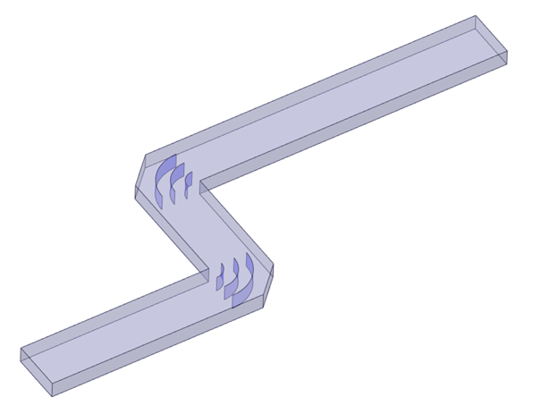
While loss coefficients can be derived via either experiment or literature, it is common to determine these coefficients via a CFD model. Since the main goal of porous media is to reduce computational complexity, naturally the whole device should not be modeled when determining these coefficients. Instead, a small “unit cell” model that fully resolves a small section of the porous geometry is used. The model has the sole purpose of generating data that will be used to determine the inertial and viscous coefficients.

The unit cell model will be run at several flow rates and the pressure drop across the model will be recorded. The velocity vs pressure drop curve formed by this data will be curve fit to the form:

Coefficients a and b will then solved for using:

Knowing that the pressure loss will always follow a parabolic curve as described above, any tuning that is perceived to be needed means that the curve fit must be altered. Similarly, if experimental testing reveals that the pressure drop vs velocity curve follows any shape other than a parabola with a y-intercept of zero, then the porous loss model cannot represent this loss accurately across, though a curve fit could potentially be done for some limited range of velocities.