How does Ansys licensing work with GPU solvers and cards?

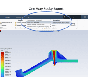
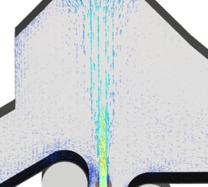
Ansys continues to develop GPU solvers as GPU based computing continues to reach maturity and shows promise as a more efficient and economical way to access powerful high-performance computing. DRD’s benchmarks show significant promise in using GPUs for computational fluid dynamics (CFD) using Fluent’s new native GPU solver and for discrete element modeling (DEM) using Ansys Rocky.

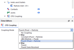
When investigating the use of GPUs to solve your complex and large problems it is important to understand the licensing implications. In this article we will discuss licensing for both Fluent and Rocky when using GPUs.

Fluent requires a CFD Enterprise license to enable the Native GPU Solver. Included in the license is the ability to use up to 40 streaming multiprocessors (SMs) on a GPU with the ability to solve on a card with a greater number of SMs by checking out HPC Workgroup or HPC Pack licenses. The table below shows the required number of HPC Workgroup tasks or HPC Packs required for a given SM count. In some sense the licensing scheme is similar to the CPU solver where HPC licensing is required to solve on more than 4 cores. Similarly, a core is a subset of the compute elements on a CPU die just like an SM is a subset of the repeating compute units on a GPU. It is important to note that an SM is not equivalent to a CUDA core. SMs contain multiple CUDA cores. This article explains how to determine the number of SMs on a given card below. It is also important to know that you must use all of the SMs on a given GPU. You cannot utilize only a portion of the SMs.

Rocky allows the use of GPUs right out of the gate with up to 112 SMs. Rocky does use it’s own HPC licensing that enables an additional 112 SMs per Rocky HPC 8 License as shown in the table below.

How Many Streaming Multiprocessors (SMs) Are on my GPU Card?

When determining how much HPC is required for a given GPU it is important to know both the target application (Fluent or Rocky) as well as the number of SMs on the card. Since you must consume all of the SMs on the card, you must have sufficient licensing to be able to invoke either solver on the card. The number of SMs on a card is rarely published, so it can seem daunting at first, but DRD has found that the website techpowerup.com readily posts the SM count. 

Search for the GPU name and “specs” in google and follow the tech powerup link:

Scrolling down to the details of the card, the SM count is listed in the “Render Config” section:

From this example, we can see that to run the Fluent native GPU solver on the RTX 4090 would require 3 HPC packs and to run Rocky on this card would require a single Rocky HPC 8 license.

DRD hopes this article helps answer questions regarding licensing of our world class GPU solvers as well as where to find published streaming multiprocessor counts for modern GPUs. Do you want to see more Ansys GPU benchmarks?  Visit our hardware page.

Bulk Material handling can frequently involve fluid flow that impacts the behavior of the particulate. Luckily, Rocky couples with Ansys Fluent to enable representation of the fluid flow and the particulate behavior. This coupling can be either one or two-way. One-way coupling solves the fluid flow first and exports the resulting flow field into Rocky. This means that particles within Rocky are affected by the flow, but the flow is not altered by the particles. In addition to a constant flow field, Rocky also supports transient one-way coupling where a time varying flow field can be imported. This can include a periodic repeating transient flow. Two-way coupling, sometimes called co-simulation, is also possible. In this configuration, Fluent and Rocky exchange information back and forth as the solution moves forward in time.   

One common application of coupling Rocky with CFD is to perform density-based separation. One application of density separation is to separate lightweight plastics from a stream of compost. In the example below, an air knife and vacuum system is used to remove the plastic from the denser wood particles.  

The first step in a one-way coupled model like this is to setup and solve the CFD model. This particular application has a low particulate loading, so one-way coupling is appropriate. The setup of this particular model included specification of the air knife and suction outlet flowrates, while specifying pressure boundaries for the clean outlet and compost inlet. Once solved, the developed flow field will be exported to Rocky using the Rocky Export tab at the top of the Fluent interface. Note that the Rocky Export tab is only available after installation of Rocky along with the Rocky coupling module. To perform a one-way export, first select Rocky Export, then Export one way data, and finally export current data to Rocky.

Once this is complete, the next step is to setup the Rocky model as normal, that is leaving the coupling setup to later. This includes importing the geometry, setting up the particle inlets and particles, etc. Finally, proceed to the CFD Coupling entry in the Data panel. In the Data Editors panel, select the appropriate coupling type. For this model, 1-Way > Fluent (Fluid -> Particle) was selected.

Following this selection, Rocky will prompt the user to select the Fluent to Rocky (.f2r) file. This is the header file of the rocky export that was performed from the Fluent interface. Note that the export performed earlier resulted in several files. An .f2r file, two .dat files and several .stl files representing each boundary in the Fluent model. You will always point to the .f2r file when referencing the export in Rocky.

Once the Fluent to Rocky file has been read in, a new entry in the Data panel will appear under the CFD coupling item. Clicking on this item will reveal settings for the one-way coupling.

Common options are to change the drag law applied to different particle shapes. The Rocky CFD Coupling Technical Manual has good advice on appropriate drag models to use. The Coloring tab of the Data Editors panel allows you to visualize the CFD data you have imported as shown below. Be sure to turn off this visualization when you are done as it can impact performance.

Finally, your model is ready to solve like normal. All of the typical postprocessing results you can expect from Rocky are still available to you, only now particles can be affected by the imported airflow. The workflow demonstrated here works well for transient or transient periodic one-way coupling as well. Two-way coupling does not rely on the Rocky Export tab in Fluent. Instead, Rocky will launch Fluent itself once provided the appropriate Case and Data files to start from.

I hope you found this short article useful. Check out our website for other Rocky and Ansys content.

Bucket conveyor models in Ansys Rocky use somewhat complex motion definitions to define the motion up the grain leg, around the head pulley, down the grain leg, and finally around the tail pulley. It is common to know the RPM of the driven pulley, so defining the motion based on this parameter is very convenient. In this post, we will demonstrate the use of expressions in Ansys Rocky to do just that. 

When setting up a bucket elevator simulation, import only a single bucket. The bucket’s mounting location should be even with the center of the tail pulley. The geometry will be replicated using the “Replicate Geometry” feature.

Next, insert a motion frame, connect the motion frame to the bucket geometry, and via the tools menu enable Expressions/Variables. The image below details the initial position of the bucket geometry and the relevant motions that must be defined. Note that based on the initial position of the bucket, there will need to be four sequential motions defined for the motion frame. These are Translation 1, Rotation 1, Translation 2, and finally Rotation 2.

These motions will be defined based on start and stop times for a given motion as well as the relevant velocity. This leads to the relevance of expressions to define the time required to perform each motion as well as the velocity based on the relevant known parameters. It is important to also note that the motion frame does not need to be in contact with the object that it is tied to. In this case it is beneficial to locate the motion frame at the center of the tail pulley. This location will make it easier to define the rotation motions.

Take the first translation as an example. The motion will start at t=0 and the bucket must traverse the distance equivalent to the center to center distance between the two pulleys, which is known to be 182.6 inches. Using the known head pulley diameter and rotational speed of 65 RPM, the linear velocity of the belt can be determined using Pi * Diam * PulleyRPM/60 as shown below.

The other required input for Translation 1 is to compute the length of time it will take the bucket to traverse the first straight section of belt. This can be computed via dividing the straight length of belt by the belt speed as shown below.

To setup Translation 1 in the motion frame, add a translation motion with a “Stop Time” equal to “StraightTime” and a velocity of “BeltSpeed” in the appropriate direction.

Note that it is important to add units to these inputs. [s] for StraightTime and [in/s] for BeltSpeed.

The next motion will require a few additional expressions. First, we will define the time to complete a semicircular rotation around the head pulley. Knowing the RPM of the pulley and that the desired motion is half of a revolution, the formula to compute the time of half a rotation simplifies to RotTime = 30/PulleyRPM. Finally, we need to determine the angular velocity. This can be computed as AngVel = -180/RotTime [dega/s]. This can be entered directly into the motions panel, or can be added as an additional Variable.

The Start and Stop Times can be defined using the StraightTime and RotTime variables already defined. The Start Time for this motion is after the end of the initial translation, therefore the start time is equal to “StraightTime.” The Stop Time is the duration of the translation and the impending rotation, so is equivalent to “StraightTime+RotTime.” The Initial Angular Velocity field is filled using the angular velocity calculation noted above.

The remaining translation and rotation motions can be defined using the same approach.

Following the remaining motion setup, the final step is to include replication of the bucket geometry. Navigating to the bucket geometry, set the Motion Frame to the frame just created and proceed to the Replication tab. Enter the number of buckets you will need and enter the replication period. The replication period is the length of time needed to complete one full loop around the conveyor. In this case it is equivalent to “2*StraightTime + 2*RotTime.”

Note that the Expressions section of the Expressions/Variables panel is a list of where expressions or variables have been used in the model.

While this article explains the setup of a bucket elevator, expressions are quite valuable for other Rocky simulations as well. When calculation is needed to convert between a key value and the inputs needed to implement that change in Rocky, expressions and aid in accuracy and speed of running multiple test cases. For this example, it is trivial to run the model at different head pulley speeds as only the PulleyRPM variable needs to be modified.

Check out our website for other tips, tricks, and Ansys content.

Boundaries in Ansys Fluent can be broken into two groups: external boundaries and internal boundaries.  External boundaries appear on the outer boundary of meshed regions (inlets, outlets, interfaces, etc.), while internal boundaries exist within a conformal mesh (interiors, porous-jumps, fans, etc.).  Notably, internal boundaries can exist inside a single cell zone, or can even separate different cell zones as long as the mesh is conformal across the boundary. There is one boundary type that can be used as either an external or internal boundary: walls.

While external walls are straight forward, internal walls are a bit more complex. Internal walls are sometimes called coupled walls or two-sided walls because they are formed by a pair of wall boundaries that are by default coupled together. You most often see coupled walls separating fluid and solid cell zones, but they can also be used as infinitely thin baffles with fluid on both sides.  Each coupled wall pair shows up in the boundary list as a zone and its shadow: one for each side of the wall.  When the coupled wall is between two different cell zones, it is easy to determine which side faces which cell zone as the adjacent cell zone is listed in the boundary condition window.

It is possible for a two-sided wall to exist between a single cell zone. When this occurs, the above reference to the “adjacent cell zone” is no longer useful to determine which side of the wall faces a particular direction. In these instances, it is possible to plot the face area in the direction most aligned with the boundary’s normal direction. The face area vector points from the adjacent cell into the wall (this is opposite of face normal direction). Note that you must initialize the solution to be able to generate the necessary contour plot.

In the below example, the “X Face Area” is plotted on the wall-baffle-shadow zone. The plot shows that the area is largely negative, which implies that this wall faces the +X direction. While this may initially seem backwards, keep in mind that the face area points from the adjacent cell towards the wall. This is backwards of the outward facing normal direction.

Hopefully this article sheds some light on wall/wall-shadow pairs. If you require further assistance with this topic, please contact us at support@drd.com.

When setting up rotating machinery in Fluent, users will specify a rotating cell zone with the appropriate angular velocity. The bounds of this domain must be surfaces of revolution for either the frame motion or sliding mesh approaches. This article focuses on the finer details of setting up such a case. Particularly, what needs to be done for walls on the boundary of a rotating zone that should not be rotating? Additionally, sometimes a rotating shaft will exist both within a rotating zone and also within an adjacent stationary zone, how should this be handled? This article will answer these questions.

As an example, consider a case where a fan is placed within a circular duct. It is held in place via the motor and motor mounts. The domain will be split into rotating and stationary zones about halfway along the shaft that connects the fan and motor assembly.

The setup of the rotating zone itself is straightforward. For this analysis, the frame motion approach will be used.  In the Cell Zone Conditions Panel, the “Frame Motion” box will be checked and the appropriate rotation axis, rotation axis direction, and rotational velocity will be set.

In Fluent, all walls are stationary relative to their adjacent cell zone. This means walls within or on a rotating zone are rotating with that zone. Similarly all walls within or on a stationary zone are stationary. Consider the two images below. The duct in the rotating cell zone should not be rotating with the fan. Conversely, the motor shaft that extends into the stationary zone should be rotating, while the cell zone should be stationary. These conditions need to be applied at the boundary level for these two walls.

The small section of shaft in the stationary zone will be treated similarly, but will instead have the same angular velocity as the rotating zone. In this model the small section of shaft in the stationary zone likely does not change the result much, but this will not always be the case.

One very important aspect of applying wall velocities as done for both the duct and the shaft is that no velocity can be applied normal to the wall. In the case of cylindrical walls, only rotational velocity around the axis of the cylinder is allowed.