The development of modern firearms and ammunition presents significant challenges. Engineers must balance performance, reliability, and safety while keeping costs and production efficiency in check. Traditional methods rely heavily on physical prototyping, which can be time-consuming and expensive. Additionally, factors such as barrel dynamics, bullet drag, thermal effects, and recoil must be optimized to ensure a firearm function effectively under various conditions.

Accuracy is one of the most critical factors in firearm performance. Barrel vibrations, thermal expansion, and rifling design all influence how precisely a bullet reaches its target. Likewise, excessive recoil can reduce shooter comfort and control, while poor thermal management in high-rate firing scenarios can cause overheating, leading to component degradation or even catastrophic failures. Understanding and mitigating these issues is essential for advancing firearm technology. This blog explores the role of physics-based simulation in firearm development and how it contributes to cutting-edge advancements in the industry.

To dive deeper into these challenges and explore solutions, join our exclusive webinar and watch our in-depth video demonstration on firearm simulation techniques.

What is Physics-Based Simulation?

Physics-based simulation involves four critical steps:

1. Providing CAD Geometry – Creating a digital model of the firearm or ammunition component.
2. Generating a Computational Mesh – Breaking down the model into smaller elements for analysis.
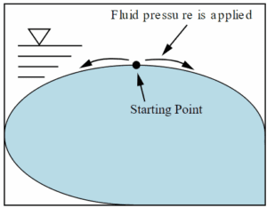
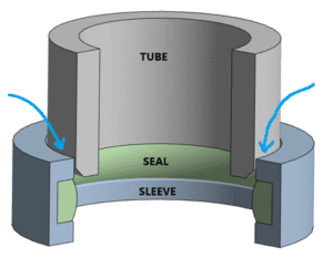
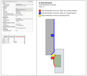
3. Setting Up Physics Parameters – Incorporating factors such as sliding friction, pressure, heat transfer, and material properties.
4. Post-Processing Results – Analyzing the simulation output to make simulation-driven design decisions.

Each type of physics—mechanical, fluid dynamics, and electromagnetics—has its own set of constitutive equations, allowing for quantitative predictions of firearm behavior.

The Role of Simulation in Firearm Development

Engineers can conduct virtual prototyping and design verification, accelerating the product development process. Simulation helps solve fundamental laws of physics, including mass, momentum, and force balances, providing insights that enhance accuracy, durability, and safety. The following are key applications of Ansys in firearm engineering.

• Barrel Dynamics and Accuracy
  

Barrel dynamics significantly impact firearm accuracy. Simulation enables engineers to tune barrel dynamics by analyzing vibrations and harmonic frequencies, ensuring minimal muzzle movement.

• Bullet Drag Prediction and Optimization
  

Predicting aerodynamic drag is crucial for improving projectile performance. Ansys simulations analyze bullet shape, rifling effects, and gas dynamics to minimize drag and enhance accuracy. By optimizing groove length and depth, engineers can achieve better flight stability and range.

• Thermal Management for High Firing Rates

Excessive heat buildup in barrels and suppressors can lead to safety risks, including accidental cook-off. Ansys simulations evaluate thermal distribution in rapid-fire scenarios, helping to mitigate overheating and structural deformation. Thermodynamics, such as non-uniform barrel heating, can also be assessed to optimize material selection and structural integrity.

• Reducing and Predicting Felt Recoil

Recoil affects shooter comfort and accuracy. Simulation allows for ergonomic analysis, studying the effects of force distribution, action delay, and muzzle devices like barrel porting or brakes to reduce perceived recoil.

• Suppressor and Muzzle Blast Characterization

Suppressors are designed to dissipate pressure waves and reduce noise. Ansys simulations predict gas expansion and pressure variations, optimizing suppressor efficiency while maintaining firearm performance.

6. Functional Testing

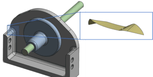
Mechanical components such as triggers, bolts, and actions require precise tolerances for smooth operation. Simulations assess tolerance stacking, material properties, and wear characteristics to ensure reliable firearm functionality before physical prototyping.

• Ballistics and Body Armor

Simulation plays a key role in assessing bullet impact on composite armor. Engineers can analyze penetration power, velocity requirements, and material resistance to improve both ammunition and protective gear designs.

Conclusion

Ansys simulation tools provide a competitive edge in firearm development by enabling precise, simulation-driven design optimizations. From improving accuracy and durability to reducing recoil and optimizing thermal management, physics-based simulations empower engineers to push the boundaries of firearm innovation. As technology continues to evolve, simulation-driven development will remain at the forefront of the industry, ensuring safer and more effective weapon systems for the future.

Want to see these simulations in action? Our webinar and video dives deep on firearm development with Ansys.

Understanding stress vs. strain is fundamental for engineers working with material properties. However, a critical distinction exists between the stress-strain data obtained during tensile tests and the true stress-strain data required for accurate simulations in software like Ansys Mechanical.

In this article, we’ll uncover the essential differences, explain how to calculate true stress and strain, and explore why these concepts are indispensable for accurate elastic-plastic material simulations.

What is Measured and Calculated During Material Tensile Testing?

If you were to internet search for a material’s stress vs. strain data or look in the back of an engineering mechanics textbook, the stress vs. strain data provided is typically in the form of engineering stress and strain. Tensile testing for stress vs. strain is performed using tensile coupons like the layout shown in Figure 1.

This layout includes data that is measured as part of the test, where:

• P = the applied load
• A = the initial cross-section area
• l₀ = the initial extensometer length
• l = the new extensometer length after applying load P

The calculated stress and strain are:

σ_engineering = P / A

ε_engineering = (l – l₀) / l₀

These are engineering stress and strain because the calculation is performed using the initial cross-section area. However, as the tensile coupon is loaded the cross-section area reduces due to the Poisson Effect. For small values of stress and strain, the difference between engineering stress and strain and true stress and strain is low and approximated as equivalent.

Determining True Stress and Strain

There’s a handy pair of equations to calculate true stress and strain using the calculated values.

σ_true = σ_eng (1+ε_eng)

ε_true = ln (1+ε_eng)

These are simple to evaluate using the engineer’s second-best tool, Excel (the first being Ansys, of course).

Why is this Distinction Important?

You may be saying to yourself, “This doesn’t seem like that big a deal. Why are you telling me this?” It’s important to understand how simulation codes perform finite element calculations.

Let’s consider a hypothetical test procedure, where we take the tensile test coupon shown in Figure 1 and stretch it from 10mm to 12mm. This is a change in length, ∆l, of 2mm. Using the equation above for engineering strain, we can calculate an engineering strain value of:

ε_engineering = 2/10 = 0.2 mm/mm

Okay… straight forward. Let’s break that up into two steps on a second tensile test coupon. Step 1 will stretch the coupon from 10mm to 11mm and step 2 will stretch it from 11mm to 12mm; then we can simply add these two strain values to get the total strain. Pretty simple, eh?

ε_engineering = 1/10 + 1/11 = 0.191 mm/mm

What you should notice is that these two measurements do not produce identical strain values, despite both tests stretching the tensile coupon the same amount. So, what does this mean for simulation?

The second tensile test, where strain is calculated in incremental stages, directly resembles how strains are calculated in Ansys Mechanical simulation from incrementally applied loads. If analysts use engineering stress and strain as input to the plasticity material models in Ansys Mechanical, each additional increment in load represents error in the strain calculation.

Let’s redo the calculation above using true strain. The third tensile test coupon:

ε_true = ln (12/10) = 0.18232 mm/mm

And the fourth:

ε_true = ln (11/10) + ln (12/11) = 0.18232 mm/mm

As you can see, we calculate identical results using true strain. This behavior is desirable in Ansys simulation and is why Ansys Mechanical requires using true stress vs. strain as input for the elastic-plastic material models.

In fact, if you peruse the Ansys Help documentation you’ll find this note:

Hmmm… this just stated what I spent ~600 words saying. That’s alright; hopefully the illustrated examples with the tensile test coupons are helpful.

Where Else Can Analysts Learn About Ansys and Plasticity?

If you are interested in learning more about Ansys and plasticity in simulation, DRD has on-demand training content on our website. This particular topic is covered in our Nonlinear Structural Simulation course, in Chapter 3.

Ansys Mechanical Nonlinear Structural Simulation – DRD Technology

Released on July 23, 2024, Ansys Mechanical 2024 R2 introduces a powerful new native feature: Fluid Penetration Pressure. While this isn’t entirely new to Ansys, as it has long been part of Ansys APDL, it’s the first time this functionality is available natively in Ansys Mechanical. This feature provides engineers with an efficient way to simulate fluid interactions with structures without explicitly modeling the fluid in finite element analysis (FEA).

What is Fluid Penetration Pressure?

Fluid pressure penetration is a method to capture impinging fluid on a structure, without explicitly modeling the fluid in the finite element analysis.

The fluid penetration pressure method employs information of contact status between contacting bodies to determine where the fluid pressure is applied. The benefit is that this is determined as the contact status evolves over the simulation time, so the region where pressure is applied changes as contact between bodies changes under loading.

Users provide a contact region for the searching algorithm, a starting location for fluid impingement, and the fluid pressure; the solver does the rest. Figure 1 provides a simple view of the starting point on the exterior surface of the structure and the ‘flow’ of the fluid outward.

Figure 1: Schematic of Fluid Penetration Pressure Behavior

What is the Application of Fluid Penetration Pressure?

As you perhaps have guessed, the application of fluid penetration pressure is in seals and gaskets for valves, hydraulic cylinders, coil-overs, etc. This allows determination of sealing surface leakage as the structure is loaded and deforms, both from the fluid pressure itself and additional loads in service.

Figure 2: Examples of Gaskets

If engineers can determine seal capability before selling the product, expensive redesign can be circumvented. Seals do not need redesign, re-machining of the sealing surfaces is lessened, and a potentially hazardous leak can be avoided.

Example Simulation with Fluid Penetration Pressure

Here we have a simple representation of a tube, sleeve and O-ring seal in a vehicle strut or coil-over. During the assembly process, the tube is pushed downward to interface with the O-ring. In service, fluid is pushing against the seal from the top in the shown orientation, annotated by the blue arrows in Figure 3. The sleeve is fixed in place.

Figure 3: Layout of Simulation with Fluid Impingement Load Direction

As stated previously, analysts need to supply a contact, a starting point, and a fluid pressure magnitude. In the 2D axisymmetric representation of the structure in Figure 3, frictional contact is defined between the three bodies. The Fluid Penetration Pressure object is defined as shown in Figure 4.

Figure 4: Example Use of Fluid Penetration Pressure Feature, Details, Load, and Graphics

As you can see, we’ve applied the fluid pressure in the second load step; the first load step is moving the tube downward.

I’ll leave you with these final output animations, and a recommendation to visit our website to get access to on-demand training.

We walkthrough this simulation example as part of our Ansys Mechanical Nonlinear Structural Simulation course. Follow the link here: Ansys Mechanical Nonlinear Structural Simulation – DRD Technology.

In our last blog post of this series, I dive into how we can simulate cracked structures using Ansys simulation software, Ansys Mechanical. As before, if you’ve not read the previous two posts, go back and read ‘em!!! 

How Engineers Use Ansys Mechanical Software to Model Cracks 

Ansys Computer Aided Engineering (CAE) simulation software allows engineers to study cracks in structures via fracture mechanics, along with a host of other structural simulation needs. Ansys has a long history of simulation development since the 1970’s in creating tools for engineers to design and virtual prototype their products. As a quick note, Ansys is not limited to just structural physics either. Fluids, electromagnetics, systems and optics are some of the other fields Ansys offers in its portfolio of simulation capabilities. 

The options to create a crack in Ansys simulation software generally fall in two categories: either a) use a CAD surface that represents the crack, that overlaps with the structure or b) use the auto-generation tool in Ansys to add a crack at the mesh level. 

The former works well in all scenarios but is very useful when the crack is not a simple analytical shape, i.e., a penny-shaped crack. The latter is great for those simple, penny-shaped cracks, where the engineer can input two radii to define the shape, input where the crack is located, and they’re done. 

Here’s an example; take this simplified cast bearing/shaft support. The machinist finds a crack when machining the bearing support housing (outlined in the blue box). Perhaps this is caused by an incorrect casting process. 

Representative CAD Model, Crack Surface on Right 

When magnafluxed or cut open, the crack is not a simple shape. This is perhaps an extreme example, but it gets the point across. With a few inputs and clicks, Ansys overlaps the crack surface with the solid CAD, splits the mesh where these intersect, buffers the elements from the new crack mesh into the existing base mesh, and voila! The finite element model crack is ready to analyze.

Representative Finite Element Mesh of Structure with Crack Inserted: Back View on Left, Top View on Right (with red line indicating part boundary) 

What About Crack Growth? 

Ansys requires no special treatment of the crack to determine the relevant fracture parameters when evaluating a crack for simple comparison to material fracture toughness. The simplicity of the Ansys workflow mirrors the simplicity of what the engineer is after, i.e., a single value for Stress Intensity Factor. Using the methods described previously, engineers can model a crack and then mesh the structure with hexahedra, tetrahedra, or a mix of element shapes and get results for Stress Intensity Factor. 

For fatigue cracks, the requirements are greater. Engineers must provide the crack growth equation constants, i.e., the Paris constants C and m, then Ansys will do the rest. Ansys’ technology for general, 3D crack growth is quite extraordinary. This technology is referred to as SMART – Separating, Morphing, and Adaptive Remeshing Technology. To put it simply, automatic remeshing occurs as the crack grows in simulation. 

Representative Crack Growth Simulation Showcasing Automated Solution Remeshing 

For a nice overview of fracture mechanics in Ansys, you can watch an on-demand webinar on DRD’s website. In the webinar, I provide a brief overview of fracture mechanics and Ansys capabilities in fracture analysis, much like this paper. I also discuss damage tolerant design, material data acquisition, and Ansys CAE simulation of cracks in structures. 

Head over to DRD’s website for two on-demand webinars I conducted in October and November, ‘Simulating Crack Propagation Part 1 and 2.’ 

https://www.drd.com/resources-all/simulating-crack-propagation-part-1-webinar-recording/ 

https://www.drd.com/resources-all/simulating-crack-propagation-part-2-webinar-recording/ 

This concludes our 3-part series on fracture mechanics. We have a few other resources engineers can dig into on this topic, including the two on-demand webinars mentioned above. DRD has a fracture mechanics training course that I teach as demand requires, https://www.drd.com/project/ansys-mechanical-fracture-mechanics/. If you are interested in this course, please let us know at support@drd.com. 

Let’s continue our discussion on fracture mechanics with this second blog post, where I dive into the methods engineers have available to evaluate cracked structures. If you’ve missed part 1 of this blog series, go back and read it here. 

Stationary, Static and Fatigue Cracks 

When evaluating a structure with cracks, engineers have a few options with respect to the level of involvement in solving the problem. From least to most involved: 

• Stationary: review of status of crack, ignoring crack growth. 
• Static: review of status of crack under single, monotonically increasing load, crack growth is assumed. 
• Fatigue: review of status of crack under cyclic loading, crack growth is assumed. 

Stationary cracks provide an instantaneous view of the state of a crack in the structure. The engineer can only know one thing from this type of analysis: will the crack grow or not. No insight is provided into the second and third of the common questions asked in the previous section. Simple closed-form solutions are available for engineers to estimate the integrity of a cracked structure, and these can be found in literature reviews and textbooks. Many closed-form solutions take the resulting stress field caused by loading, the current crack length, and an empirically determined factor to determine stress intensity. A few examples are shown here, for plate geometry of varying sizes. 

Image Source: Elementary Engineering Fracture Mechanics, 4th Ed., Broek, pg. 85 

Static cracks allow the engineer to determine if a crack will grow and fast fracture, or if the crack will arrest. Static cracks are subjected to a single, increasing load, from unloaded to fully loaded. In this case, we are not interested in a time frame for the crack to grow or arrest; ultimately, engineers simply determine if the structure will break with the presence of the crack. 

Fatigue cracks, or fatigue crack growth, is the most complex case, both for understanding and to consider when designing a product. Fatigue crack growth considers the structure under cyclic loading, where the structure is repeatedly loaded and unloaded. There are variations to this load pattern as well, which we will not go into here. 

When it comes to fatigue cracks, there are additional test procedures to determine a crack growth rate versus the applied stress intensity. Engineers will typically see this abbreviated as da/dN vs. dK, i.e., the change in crack extension (da) over cycles per extension (dN) vs. change in stress intensity (dK). Like critical fracture toughness, every material will have a different crack growth curve. Examples of some different material curves are shown here. 

Image Source: Effects of ductile laminate thickness, volume fraction, and orientation on fatigue-crack propagation in Ti-Al3Ti metal-intermetallic laminate composites, Adharapurapa et al, 2005. 

The unique aspect of fatigue crack growth that harkens back to what Griffith found is the stress levels in the structure can be much less than those that would normally cause plastic collapse. Cyclically loading the structure will continue to grow the crack, under no threat of plastic collapse, and when the maximum stress intensity factor is less than the critical fracture toughness; we call this subcritical crack growth. 

Most crack growth data focus on this subcritical crack region, however, two other regions exist. Let’s limit the data shown in the previous graph to one material’s data set and expand the representative data out; we get a graph that looks like this. 

Image Source: A review of fatigue crack propagation modelling techniques using FEM and XFEM, Rege et al, 2017. 

The material data mentioned fits into the area marked ‘Region II’; on a log-log plot of crack growth rate versus change in stress intensity, this is commonly referred to as the Paris regime, and it is generally a straight line on this plot. A simple equation is used to describe this region, which takes the form of: 

where C and m are material constants determined via the graphed data. The other two regions, I and III, refer to the threshold and fast fracture regions, respectively. The threshold region describes when the crack grows slowly, either by small stress intensity or small crack size. Conversely, the fast fracture region describes rapid crack growth, which may result in surprise failure of the structure. Engineers use this crack growth data in damage tolerance assessment. 

In both the first and second blog posts, I’ve not touched on Ansys simulation to solve fracture mechanics problems. In the next blog post, I will discuss Ansys’ capability to model cracks and solve crack growth problems.