How to Troubleshoot Failed Solves in Ansys Mechanical: A Step-by-Step Guide
When you initiate a solve in Ansys Mechanical, the program attempts to find a solution based on the boundary conditions you’ve specified. However, not all problems will solve on the first attempt. This guide will show you how to use Ansys Mechanical’s troubleshooting tools to resolve failed solves and produce accurate results.
How to Identify a Failed Solve
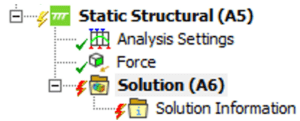
A failed solve is indicated by a red lightning bolt next to the solution. When this happens, Ansys generates error messages that explain what went wrong.
By clicking the Messages button, you can view a list of these messages categorized as Info, Warning, or Error. Warning messages should be read and understood, but they do not always indicate a problem. Error messages are generated when solving (or another action) fails to complete, and these messages explain what happened. You will need to address the cause of the error message before proceeding. Later in this article, we will recommend troubleshooting steps for the most common errors.
![]()
![]()
- Warnings: Indicate potential issues but may not affect the solve.
- Errors: Must be addressed as they prevent the solve from completing.
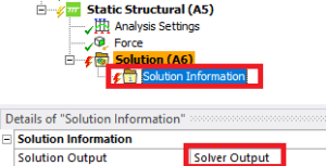
Using the Solution Information Worksheet
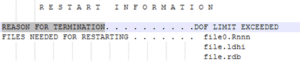
To further troubleshoot, search the Solution Information worksheet for terms like “error” or “reason for termination.” These messages provide specific details on why the solve failed. Understanding when the failure occurred (e.g., which load steps were completed) is also crucial for narrowing down the issue.
Use CTRL+F to search for “error” and read any error messages you find here. Sometimes there will be more detailed messages here. The last error message is usually the ultimate reason the solve failed.
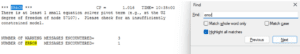
Also search for the phrase “reason for termination.” If present, this line indicates exactly why the solve failed. Recommendations for interpreting some of the common reasons for termination are described later in this article.
Next, figure out when the solve failure occurred. It is important to know what load steps, if any, were completed before the solve terminated because that will narrow down the cause. For instance, if no time points were solved, the problem may be that the model is initially underconstrained. If the solve completed two load steps and failed on the third, you should look at any changes to the boundary conditions in the third load step.
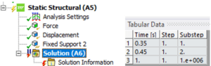
Select Solution and view the Tabular Data as shown below. This shows that two substeps were solved, and the last successful step was t = 0.45s. The third row that shows Substep = 1e+006 represents the unconverged results and does not mean that t = 1s solved successfully. It can be very informative to create result plots set to the last converged substeps (t = 0.45s in the example below). The results at unconverged substeps are not physically meaningful and should generally not be used.
Once you understand the error that terminated the solve and the load step when the solve terminated, you can take corrective action to make the solve successful. The next steps will depend on the error encountered. For detailed advice, see DRD’s blog on troubleshooting steps based on the most common error messages.
Troubleshooting Tips
- Check constraints: Ensure all parts are sufficiently constrained to prevent rigid body motion (RBM).
- Review boundary conditions: If the solve failed after completing a load step, inspect changes in boundary conditions.
- Create result plots: Use the last converged substep to identify potential issues. Unconverged substep results are not physically meaningful and should generally be ignored.
Want to dig deeper into advanced troubleshooting? Our blog on using Ansys Mechanical diagnostic tools covers additional tips to help you streamline your solving process