Using Ansys Mechanical Software to Model Cracks (Part 3 of 3 in a series on Fracture Mechanics)

In our last blog post of this series, I dive into how we can simulate cracked structures using Ansys simulation software, Ansys Mechanical. As before, if you’ve not read the previous two posts, go back and read ‘em!!! 

How Engineers Use Ansys Mechanical Software to Model Cracks 

Ansys Computer Aided Engineering (CAE) simulation software allows engineers to study cracks in structures via fracture mechanics, along with a host of other structural simulation needs. Ansys has a long history of simulation development since the 1970’s in creating tools for engineers to design and virtual prototype their products. As a quick note, Ansys is not limited to just structural physics either. Fluids, electromagnetics, systems and optics are some of the other fields Ansys offers in its portfolio of simulation capabilities. 

The options to create a crack in Ansys simulation software generally fall in two categories: either a) use a CAD surface that represents the crack, that overlaps with the structure or b) use the auto-generation tool in Ansys to add a crack at the mesh level. 

The former works well in all scenarios but is very useful when the crack is not a simple analytical shape, i.e., a penny-shaped crack. The latter is great for those simple, penny-shaped cracks, where the engineer can input two radii to define the shape, input where the crack is located, and they’re done. 

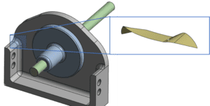
Here’s an example; take this simplified cast bearing/shaft support. The machinist finds a crack when machining the bearing support housing (outlined in the blue box). Perhaps this is caused by an incorrect casting process. 

Representative CAD Model, Crack Surface on Right 

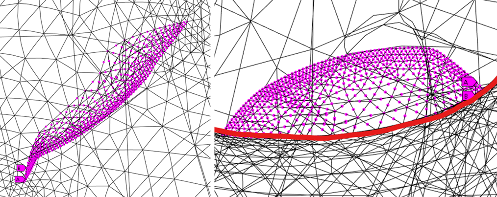
When magnafluxed or cut open, the crack is not a simple shape. This is perhaps an extreme example, but it gets the point across. With a few inputs and clicks, Ansys overlaps the crack surface with the solid CAD, splits the mesh where these intersect, buffers the elements from the new crack mesh into the existing base mesh, and voila! The finite element model crack is ready to analyze.

Representative Finite Element Mesh of Structure with Crack Inserted: Back View on Left, Top View on Right (with red line indicating part boundary) 

What About Crack Growth? 

Ansys requires no special treatment of the crack to determine the relevant fracture parameters when evaluating a crack for simple comparison to material fracture toughness. The simplicity of the Ansys workflow mirrors the simplicity of what the engineer is after, i.e., a single value for Stress Intensity Factor. Using the methods described previously, engineers can model a crack and then mesh the structure with hexahedra, tetrahedra, or a mix of element shapes and get results for Stress Intensity Factor. 

For fatigue cracks, the requirements are greater. Engineers must provide the crack growth equation constants, i.e., the Paris constants C and m, then Ansys will do the rest. Ansys’ technology for general, 3D crack growth is quite extraordinary. This technology is referred to as SMARTSeparating, Morphing, and Adaptive Remeshing Technology. To put it simply, automatic remeshing occurs as the crack grows in simulation. 

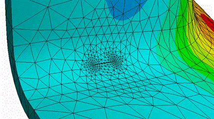
Representative Crack Growth Simulation Showcasing Automated Solution Remeshing 

For a nice overview of fracture mechanics in Ansys, you can watch an on-demand webinar on DRD’s website. In the webinar, I provide a brief overview of fracture mechanics and Ansys capabilities in fracture analysis, much like this paper. I also discuss damage tolerant design, material data acquisition, and Ansys CAE simulation of cracks in structures. 

Head over to DRD’s website for two on-demand webinars I conducted in October and November, ‘Simulating Crack Propagation Part 1 and 2.’ 

https://www.drd.com/resources-all/simulating-crack-propagation-part-1-webinar-recording/ 

https://www.drd.com/resources-all/simulating-crack-propagation-part-2-webinar-recording/ 

This concludes our 3-part series on fracture mechanics. We have a few other resources engineers can dig into on this topic, including the two on-demand webinars mentioned above. DRD has a fracture mechanics training course that I teach as demand requires, https://www.drd.com/project/ansys-mechanical-fracture-mechanics/. If you are interested in this course, please let us know at support@drd.com. 

Methods for Engineers to Evaluate Cracks (Part 2 of 3 in a series on Fracture Mechanics)

Let’s continue our discussion on fracture mechanics with this second blog post, where I dive into the methods engineers have available to evaluate cracked structures. If you’ve missed part 1 of this blog series, go back and read it here. 

Stationary, Static and Fatigue Cracks 

When evaluating a structure with cracks, engineers have a few options with respect to the level of involvement in solving the problem. From least to most involved: 

  • Stationary: review of status of crack, ignoring crack growth. 
  • Static: review of status of crack under single, monotonically increasing load, crack growth is assumed. 
  • Fatigue: review of status of crack under cyclic loading, crack growth is assumed. 

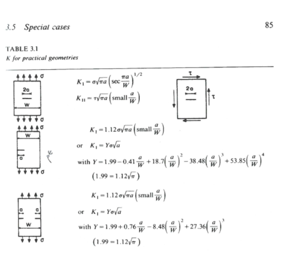
Stationary cracks provide an instantaneous view of the state of a crack in the structure. The engineer can only know one thing from this type of analysis: will the crack grow or not. No insight is provided into the second and third of the common questions asked in the previous section. Simple closed-form solutions are available for engineers to estimate the integrity of a cracked structure, and these can be found in literature reviews and textbooks. Many closed-form solutions take the resulting stress field caused by loading, the current crack length, and an empirically determined factor to determine stress intensity. A few examples are shown here, for plate geometry of varying sizes. 

Static cracks allow the engineer to determine if a crack will grow and fast fracture, or if the crack will arrest. Static cracks are subjected to a single, increasing load, from unloaded to fully loaded. In this case, we are not interested in a time frame for the crack to grow or arrest; ultimately, engineers simply determine if the structure will break with the presence of the crack. 

Fatigue cracks, or fatigue crack growth, is the most complex case, both for understanding and to consider when designing a product. Fatigue crack growth considers the structure under cyclic loading, where the structure is repeatedly loaded and unloaded. There are variations to this load pattern as well, which we will not go into here. 

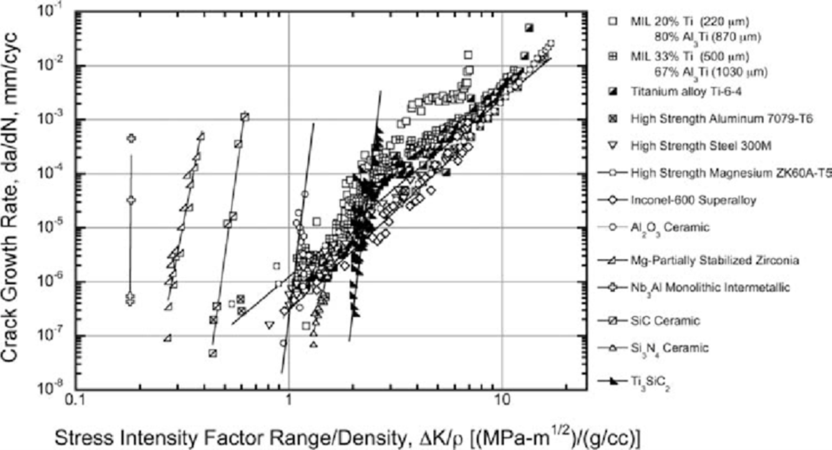
When it comes to fatigue cracks, there are additional test procedures to determine a crack growth rate versus the applied stress intensity. Engineers will typically see this abbreviated as da/dN vs. dK, i.e., the change in crack extension (da) over cycles per extension (dN) vs. change in stress intensity (dK). Like critical fracture toughness, every material will have a different crack growth curve. Examples of some different material curves are shown here. 

The unique aspect of fatigue crack growth that harkens back to what Griffith found is the stress levels in the structure can be much less than those that would normally cause plastic collapse. Cyclically loading the structure will continue to grow the crack, under no threat of plastic collapse, and when the maximum stress intensity factor is less than the critical fracture toughness; we call this subcritical crack growth. 

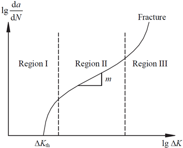
Most crack growth data focus on this subcritical crack region, however, two other regions exist. Let’s limit the data shown in the previous graph to one material’s data set and expand the representative data out; we get a graph that looks like this. 

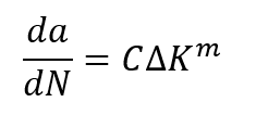
The material data mentioned fits into the area marked ‘Region II’; on a log-log plot of crack growth rate versus change in stress intensity, this is commonly referred to as the Paris regime, and it is generally a straight line on this plot. A simple equation is used to describe this region, which takes the form of: 


where C and m are material constants determined via the graphed data. The other two regions, I and III, refer to the threshold and fast fracture regions, respectively. The threshold region describes when the crack grows slowly, either by small stress intensity or small crack size. Conversely, the fast fracture region describes rapid crack growth, which may result in surprise failure of the structure. Engineers use this crack growth data in damage tolerance assessment. 

In both the first and second blog posts, I’ve not touched on Ansys simulation to solve fracture mechanics problems. In the next blog post, I will discuss Ansys’ capability to model cracks and solve crack growth problems. 

The Motivation and Method to Study Cracks in Structures (Part 1 of 3 in a series on Fracture Mechanics)

Before we jump into the topic at hand, I’d like to introduce myself. My name is Alex Austin, and I am the Structural Team Lead at DRD Technology, an Ansys Channel Partner. I studied Mechanical Engineering at the University of Tulsa, OK, from which I graduated with a BS and MS in Mechanical Engineering a little over a decade ago (woo… it’s already been that long!). My graduate work was in the fatigue and fracture space. My primary area of expertise is structural mechanics; as many engineers may know, this is quite a large field of physics when we look at Ansys simulation capabilities. Fracture mechanics is a small part of that overall field, is relatively new in the world of engineering, and is very complex. 

What is Fracture Mechanics? 

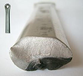
When engineers evaluate stress in a structure, the common, simple equation that comes to mind is stress = force/area. This equation carries several assumptions: static equilibrium, uniform cross-sectional area, uniaxial stress, to name a few. With the introduction of a crack to the structure, the state of stress at the crack tip is not uniaxial. Cracks are sharp corners, or notches. In the computer simulation (finite element) world, we call these singularities. In fact, singularities are locations where the theoretical stress is infinite. A strength of materials approach does not account for these singularities. When a crack exists, we need a method to analyze it. Fracture mechanics is that method. Fracture mechanics is the study of crack propagation in materials. 

Image Source: Wikipedia 

Motivation for Fracture Mechanics 

Often, cracks naturally form during the manufacturing process, either through casting or machining methods. Cracks can exist in a product and never cause issues with the working of the structure. In fact, cracks may be invisible to the naked eye. However, when this is not the case, what happens? 

Let’s say we’ve designed and manufactured structure that is currently out in the field, and our customer notices a crack… is this a problem? Let’s say a customer reported cracks popping up on some rotating machinery housings and they simply asked, ‘Is this a problem?’ though, the more likely case is no questions and, ‘Please fix this!!!’. What is the engineer typically tasked with determining? The common questions we ask are: 

  1. Will the crack grow? If so, 
  1. How quickly will the crack grow? And then, 
  1. Will the structure fail catastrophically? 

As stated, the customer absolutely thinks the presence of a crack is a problem. This is commonly the case when the customer is not an engineer, and even if they’re an engineer, they had no insight into the design and manufacture of the product. Answering the above questions will directly determine if the crack is or is not a problem. 

What about the case where the engineer designs a structure and during the design process must consider a structure that has cracks? This is a common practice in regulatory bodies, namely, the FAA (Federal Aviation Administration). In this case, the engineer assumes a crack or cracks exist in the designed components and must design for this potential failure mode. This is referred to as Fatigue and Damage Tolerance. The engineer establishes inspection intervals for components based on this analysis. The maintenance crew knows how many hours the component can be used before it needs to be checked for integrity and possibly replaced. 


In the next blog post, we will discuss the methods to evaluate cracked structures. 


Discovering New Possibilities With Ansys Discovery (and is SpaceClaim going away??)

If you’ve paid attention to new and emerging technologies in the world of simulation, you may be wondering, “What’s all this hype about Ansys Discovery?” In this blog, we will help answer this question by discussing some of the key features in Discovery, as well as what the future holds for current SpaceClaim users.

Is Discovery Modeling replacing SpaceClaim?

The older SpaceClaim interface has joined DesignModeler as a maintenance mode product in 2023R2. This means the SpaceClaim GUI will continue to be available, and Ansys will continue to perform major bug fixes. However, all new modeling capabilities are being developed within the Ansys Discovery Modeling interface.

How does the new license structure work?

The Discovery Modeling license give you access to all 3 of Ansys’ modeling applications:

  • Discovery Modeling (Simulation comes with Discovery Simulation license)
  • SpaceClaim
  • DesignModeler

Discovery Modeling and SpaceClaim can also be accessed through Enterprise or PrepPost bundles


SpaceClaim and DesignModeler standalone licenses have been discontinued

Benefits of Switching to Discovery Modeling

I already use SpaceClaim, why should I consider learning Discovery Modeling?

If you are a SpaceClaim user, you may be wondering if it is worth your while to switch to something new. Before we dive into new features of the Discovery Modeling package, let’s talk about what this transition actually looks like:

  • With Discovery Modeling license, you can simply open your existing SpaceClaim geometry in Discovery from the workbench page and pick up your projects right where you left off.


If you’re starting a new model from scratch, Discovery continues to support direct import of major external CAD formats.


  • Discovery gives you access to the same features you love from SpaceClaim with a new and improved UI. Ie, Familiar tools with new and improved functionality.

Still intimidated by the new look? Discovery has a plethora of online training materials, as well as tutorials and documentation baked into the application so you can spend less time learning a new interface and more time getting work done. You can also check out DRD’s Discovery learning page for more information.

Ok, Ok, But is Discovery Modeling actually better than SpaceClaim?

So far we’ve covered that Discovery Modeling is highly accessible to existing SpaceClaim users, but is it actually better? We could spend all day discussing the various reasons people are switching to Discovery Modeling, but here are a few of the highlights:

1) Advanced Geometry Cleanup

Clean up models faster in Discovery Modeling with more built in repair and detection features.

2) Advanced Model Prep

Create Beam connections for bolted connections with ease. Model pretension directly in the Discovery GUI, or transfer the connections to Mechanical for higher fidelity solutions.

3) Sub-D

Whether you’re working with 3D scans or geometry generated by Discovery’s topology optimization tool, Designers can say goodbye to STL manipulation headaches with the all new Sub-D modeling. This feature enables interactive organic editing you’ll have to see to believe.

4) Simulation that Just Works

Unlike SpaceClaim, the Discovery GUI goes beyond being just an advanced geometry preprocessing tool by giving designers access to easy-to-use simulation across multiple physics (if Discovery Simulation is licensed). Discovery’s GPU based solvers provide immediate feedback on geometry changes in real time. Need higher fidelity? You can even submit simulations to the flagship Fluent or Mechanical solvers without leaving the Discovery environment.

If you have questions about transitioning from SpaceClaim to Discovery Modeling, one of our experienced staff would love to chat. Contact DRD today to see if Discovery is right for your team!

Rocky One Way CFD Coupling

Bulk Material handling can frequently involve fluid flow that impacts the behavior of the particulate. Luckily, Rocky couples with Ansys Fluent to enable representation of the fluid flow and the particulate behavior. This coupling can be either one or two-way. One-way coupling solves the fluid flow first and exports the resulting flow field into Rocky. This means that particles within Rocky are affected by the flow, but the flow is not altered by the particles. In addition to a constant flow field, Rocky also supports transient one-way coupling where a time varying flow field can be imported. This can include a periodic repeating transient flow. Two-way coupling, sometimes called co-simulation, is also possible. In this configuration, Fluent and Rocky exchange information back and forth as the solution moves forward in time.   

One common application of coupling Rocky with CFD is to perform density-based separation. One application of density separation is to separate lightweight plastics from a stream of compost. In the example below, an air knife and vacuum system is used to remove the plastic from the denser wood particles.  

The first step in a one-way coupled model like this is to setup and solve the CFD model. This particular application has a low particulate loading, so one-way coupling is appropriate. The setup of this particular model included specification of the air knife and suction outlet flowrates, while specifying pressure boundaries for the clean outlet and compost inlet. Once solved, the developed flow field will be exported to Rocky using the Rocky Export tab at the top of the Fluent interface. Note that the Rocky Export tab is only available after installation of Rocky along with the Rocky coupling module. To perform a one-way export, first select Rocky Export, then Export one way data, and finally export current data to Rocky.


Once this is complete, the next step is to setup the Rocky model as normal, that is leaving the coupling setup to later. This includes importing the geometry, setting up the particle inlets and particles, etc. Finally, proceed to the CFD Coupling entry in the Data panel. In the Data Editors panel, select the appropriate coupling type. For this model, 1-Way > Fluent (Fluid -> Particle) was selected.


Following this selection, Rocky will prompt the user to select the Fluent to Rocky (.f2r) file. This is the header file of the rocky export that was performed from the Fluent interface. Note that the export performed earlier resulted in several files. An .f2r file, two .dat files and several .stl files representing each boundary in the Fluent model. You will always point to the .f2r file when referencing the export in Rocky.


Once the Fluent to Rocky file has been read in, a new entry in the Data panel will appear under the CFD coupling item. Clicking on this item will reveal settings for the one-way coupling.


Common options are to change the drag law applied to different particle shapes. The Rocky CFD Coupling Technical Manual has good advice on appropriate drag models to use. The Coloring tab of the Data Editors panel allows you to visualize the CFD data you have imported as shown below. Be sure to turn off this visualization when you are done as it can impact performance.


Finally, your model is ready to solve like normal. All of the typical postprocessing results you can expect from Rocky are still available to you, only now particles can be affected by the imported airflow. The workflow demonstrated here works well for transient or transient periodic one-way coupling as well. Two-way coupling does not rely on the Rocky Export tab in Fluent. Instead, Rocky will launch Fluent itself once provided the appropriate Case and Data files to start from.

I hope you found this short article useful. Check out our website for other Rocky and Ansys content.


Plotting Cross-Sectional Averaged Values: Part 2 – EnSight

As mentioned in Part 1 of this blog, you reduce complex 3D flows down to cross-sectional averaged values for plotting against the distance along the flow path in either of Ansys’s dedicated post-processing tools: CFD-Post and EnSight.  Part 2 of this blog will focus on the method available in EnSight.

Method 3: Query

Application: Ansys EnSight

Pro: Utilizes EnSight, which can be used for much larger models than is practical with CFD-Post

Con: Defining cross-section location can be very difficult for complex geometry

EnSight’s Query tool has a built-in feature for cycling a location over a range of values, performing a calculation as it progresses, and making a plot of that data.

The first step to use this feature is to create a location that defines the cross-section of your flow path.  For simple geometry this will just be a Clip along a particular direction, but for more complicated flow paths this could involve defining a spline path for a clip to follow.

Next, you will need to create a Variable that calculates the cross-sectional average of the quantity of interest on the clip.  For transported quantities, this should be a mass-flow-weighted average.  Unfortunately, EnSight does not have a direction-independent mass-flow-weighted average function, but one can be built in a few steps.  First, a new variable for mass flux needs to be created.

Then, the weighted average can be calculated on the clip using the SpaMeanWeighted predefined function and the MassFlux variable that was created in the previous step.

To create the plot of the averaged value as the clip progresses along the flow path, create a new Query using Query > Over time/distance, set the Sample to By constant on part sweep, select the variable that was just created, Start, set the range and number of samples, and then Create query.

Note that the plot data can be exported to a file by right-clicking on the query and choosing Data > Save CSV file.

Plotting Cross-Sectional Averaged Values: Part 1 – CFD-Post

When analyzing complex 3D flow, it’s often helpful to visualize data using simple 1D plots.  One of the most commonly requested plots is to be able to show how the flow is changing on average as you progress from inlet to outlet.  While there is a native feature in Ansys Fluent to calculate circumferential averages on boundaries and plot them with respect to the axial direction (for reference, the TUI command /plot circum-avg-axial), for volumetric data this process needs to be done in one of the dedicated post-processing tools: CFD-Post or EnSight.  This blog will show various methods to create cross-sectional average plots within each tool as well as discuss some of the pros and cons of each method.

Part 1 focuses on the two methods available in CFD-Post.

Method 1: Turbo Mode

Application: Ansys CFD-Post

Pro: Easiest method to enable and customize

Con: Limited to axially-aligned geometry

CFD-Post has a suite of turbomachinery focused post-processing tools called Turbo Mode.  However, it is not limited to just turbomachinery models.  To utilize Turbo Mode, you simply have to identify a hub, shroud, inlet, and outlet.  If those items exist as part of your geometry, you can just specify them directly, but if not you can identify them using a series of Lines.  For example, you can create a hub line along the axis of your model, a shroud line around the outer diameter, and then inlet and outlet lines to connect the two.

Note that for the purposes of calculating average data the lines do not have to follow the exact contour of the geometry.

Once this is done, within Turbo Mode you can identify the global rotation axis (the axis perpendicular to your cross-section), specify the Lines that were just created, and Initialize.  This will create a 2D grid defining the revolved region for the calculations.

Now that the region has been identified, you can use the Inlet to Outlet chart to plot area-weight or mass-flow-weighted values versus progress from inlet to outlet.

Method 2: Scripting a Session File

Application: Ansys CFD-Post

Pro: Direct control over process, allowing for complex flow paths

Con: Requires knowledge of CFX Command Language and Perl

The most direct way of getting cross-sectional averaged values along a flow path is to create a location that defines the cross-section, calculate the averaged value at that location, and then script the progression of the location from inlet to outlet.  In CFD-Post, this scripting is done using Sessions.

First, a location needs to be created: typically a simple plane, but if the flow path is complex then a bounded plane defined by point and normal.

Then, an Expression needs to be created that calculates the appropriate type of average on the plane, such as area-weighted or mass-flow-weighted.

To start the scripting process, you will need the code to modify the plane location.  This can be generated by starting a new Session, starting Recording, editing the plane location, and then stopping the Recording.  This creates a CSE file in your working directory.

The CSE file can then be modified with Perl commands to loop over the flow path from inlet to outlet and save the calculated Expression value to a file.  Once that is done, the modified Session file can then be played back in CFD-Post to perform the calculations.

An example of this script can be obtained by e-mailing support@drd.com

Simplify Setup of Bucket Conveyor Models in Ansys Rocky Using Expressions

Bucket conveyor models in Ansys Rocky use somewhat complex motion definitions to define the motion up the grain leg, around the head pulley, down the grain leg, and finally around the tail pulley. It is common to know the RPM of the driven pulley, so defining the motion based on this parameter is very convenient. In this post, we will demonstrate the use of expressions in Ansys Rocky to do just that. 

When setting up a bucket elevator simulation, import only a single bucket. The bucket’s mounting location should be even with the center of the tail pulley. The geometry will be replicated using the “Replicate Geometry” feature.

Next, insert a motion frame, connect the motion frame to the bucket geometry, and via the tools menu enable Expressions/Variables. The image below details the initial position of the bucket geometry and the relevant motions that must be defined. Note that based on the initial position of the bucket, there will need to be four sequential motions defined for the motion frame. These are Translation 1, Rotation 1, Translation 2, and finally Rotation 2.


These motions will be defined based on start and stop times for a given motion as well as the relevant velocity. This leads to the relevance of expressions to define the time required to perform each motion as well as the velocity based on the relevant known parameters. It is important to also note that the motion frame does not need to be in contact with the object that it is tied to. In this case it is beneficial to locate the motion frame at the center of the tail pulley. This location will make it easier to define the rotation motions.

Take the first translation as an example. The motion will start at t=0 and the bucket must traverse the distance equivalent to the center to center distance between the two pulleys, which is known to be 182.6 inches. Using the known head pulley diameter and rotational speed of 65 RPM, the linear velocity of the belt can be determined using Pi * Diam * PulleyRPM/60 as shown below.


The other required input for Translation 1 is to compute the length of time it will take the bucket to traverse the first straight section of belt. This can be computed via dividing the straight length of belt by the belt speed as shown below.


To setup Translation 1 in the motion frame, add a translation motion with a “Stop Time” equal to “StraightTime” and a velocity of “BeltSpeed” in the appropriate direction.


Note that it is important to add units to these inputs. [s] for StraightTime and [in/s] for BeltSpeed.

The next motion will require a few additional expressions. First, we will define the time to complete a semicircular rotation around the head pulley. Knowing the RPM of the pulley and that the desired motion is half of a revolution, the formula to compute the time of half a rotation simplifies to RotTime = 30/PulleyRPM. Finally, we need to determine the angular velocity. This can be computed as AngVel = -180/RotTime [dega/s]. This can be entered directly into the motions panel, or can be added as an additional Variable.

The Start and Stop Times can be defined using the StraightTime and RotTime variables already defined. The Start Time for this motion is after the end of the initial translation, therefore the start time is equal to “StraightTime.” The Stop Time is the duration of the translation and the impending rotation, so is equivalent to “StraightTime+RotTime.” The Initial Angular Velocity field is filled using the angular velocity calculation noted above.


The remaining translation and rotation motions can be defined using the same approach.

Following the remaining motion setup, the final step is to include replication of the bucket geometry. Navigating to the bucket geometry, set the Motion Frame to the frame just created and proceed to the Replication tab. Enter the number of buckets you will need and enter the replication period. The replication period is the length of time needed to complete one full loop around the conveyor. In this case it is equivalent to “2*StraightTime + 2*RotTime.”


Note that the Expressions section of the Expressions/Variables panel is a list of where expressions or variables have been used in the model.


While this article explains the setup of a bucket elevator, expressions are quite valuable for other Rocky simulations as well. When calculation is needed to convert between a key value and the inputs needed to implement that change in Rocky, expressions and aid in accuracy and speed of running multiple test cases. For this example, it is trivial to run the model at different head pulley speeds as only the PulleyRPM variable needs to be modified.

Check out our website for other tips, tricks, and Ansys content.


Software Simulation vs. Traditional Prototyping: Accelerating Product Development with Risk-Free Testing


Introduction

In the ever-evolving world of product development for all kinds of industries including aviation, automotive, manufacturing, and healthcare, engineers face many challenges while developing a final product that meets requirements. Both physical prototyping and software simulation help engineers model and analyze different systems, processes, and products. Understanding the differences between these two methods becomes crucial for developing products on-time and on-spec. In this blog, we’ll explore the distinctions between traditional prototyping and software simulation to help you choose the right path for your project.

Physical Prototyping

The setup and integrations required for physical prototyping consists of having design software, materials, test equipment and techniques, and quality assurance. The materials will vary depending on the nature of the project but can include raw materials, electronic components, or mechanical parts. Having the proper equipment also requires the right safety equipment to ensure a safe working environment.


Software Simulation

The setup and integrations required for software simulations depend on a few common elements and considerations. Hardware must be capable of running the simulation software with sufficient processing power and memory, and software should be selected based on specific features for your simulation. Lastly, training and support materials for users and developers are helpful for long-term success.

Both software simulation and physical prototyping have a place in the product development cycle. These two approaches serve different but complementary purposes within the product development process. Engineers must determine how much physical testing can be avoided through the use of software simulation during product development.  With the understanding of cost, time, and product requirements, they can choose the best path to ensure that the final product meets the desired specifications and quality standards.

Cost Considerations Drive Decisions

Software simulation may result in a higher initial investment in terms of software and training. These upfront costs are associated with developing or implementing a simulation software system for a specific purpose. Many simulation products come with licensing or subscription fees that can be one-time, monthly, or an annual renewal cost. However, software simulations generally have a lower long-term cost and reduce the need for physical materials, machinery, and labor that are necessary for physical testing. For applications where upfront cost is the absolute deciding factor, physical prototyping can be the right solution. For organizations looking to invest in their product development cycle, simulation provides a long-term solution that can be used repeatedly as you modify and evolve a product or create new products.

Speed

Time to market is a critical factor for many projects across all industries. It is based on the scope and complexity of the project, the team’s experience with software, and access to all resources required to complete the project. Simulation provides a digital platform that invites collaboration for sharing, analyzing, and discussions. It is more accessible to work collaboratively across distances saving time than requiring physical presence, which can create logistical challenges.

Risk assessments are paramount in product development. Simulation can help identify potential risks and issues early in the process, saving time and resources. The common risks and challenges associated with simulation varies from the quality of data input, the possibility of bugs or limitations in software tools to produce inaccurate results, and ensuring the model accurately fits the real-world representation. When time is not a critical factor for projects, physical prototyping is often used in product development. One would have the ability to physically interact with the product quickly, giving you a real-world sense of its form, function, and usability. Simulation abates the need for physical components – when supply chain constraints are an issue, engineers using simulation can begin testing based on the software-defined version of their product rather than having to wait for physical prototypes.


End Product Variables

Building physical prototypes can be expensive if numerous iterations are required.  Several types of products and industries often involve more than one iteration due to the complexity and need for optimization. In the electronics industry, products like smartphones and laptops undergo frequent iteration to incorporate the latest improvement and enhance user experience. In the Aerospace industry, complex systems like aircraft and satellites require extensive iterations to meet the strict guidelines. Car manufacturers and development of medical devices to name a few more.

Software simulation allows for rapid testing and iterations as many changes can be made virtually with a few clicks. This allows for quick changes and adjustments without the need to rebuild physical models. The flexibility to develop multiple iterations saves both time and resources. In contrast, physical prototyping may require more time and resources through each iteration. While physical prototyping for real-world testing is a crucial phase in product development, ideally it would be limited due to the time and costs involved. In addition, during real-world testing, unexpected issues or challenges can arise that are native only to the test environment.

Nelson Global harnessed the power of software simulation in this real-world example to optimize their muffler designs for refrigerated transport vehicles. By leveraging simulation, Nelson Global significantly reduced development time and costs, all while enhancing efficiency, reducing emissions, and meeting regulatory requirements. Nelson Global used the Ansys software suite to design two mufflers within three days. The typical duration for physical prototyping would be weeks involving manual hand calculations with less of an accurate outcome. 

In the end, both software simulation and physical prototyping have their places in product development. For many, a combination of both approaches can be the most effective solution. Starting with software simulation for the initial design and risk assessment, and then transitioning to physical prototyping for real-world testing. The right approach is the one that will align with your project’s requirements. 

The combination of Ansys, a globally recognized simulation tool, and DRD Technology, an integrator for Ansys tools, offer a comprehensive approach to product design and optimization. Ansys provides a suite of engineering simulation software tools that are widely used in various industries to simulate real-world scenarios. Ansys software simulation includes but is not limited to structures, fluid dynamics, electromagnetics, optical simulation, acoustic, and thermal analysis. These tools can be used in a wide range of industries including aerospace, automotive, electronics, manufacturing, and many more. Ansys Elite Channel Partner, DRD Technology, has achieved the highest level of proficiency and met rigorous performance requirements with the Ansys platform so that we can help you design, simulate, and succeed.


To learn more, read the full case study documenting how Nelson Global took their prototyping process from weeks to just three days using simulation.

Working with Faceted Geometry in Ansys Fluent Meshing

Faceted geometry comes in several different formats with OBJ, PLY, and STL being commonly used.  Some simulation tools require solid geometry before importing.  Fortunately, Fluent Meshing is designed to work with surface models. These faceted file formats are often the standard when working with 3D scanned geometry in the medical community and in the field of additive manufacturing. Faceted geometry approximates a geometric shape by representing it as a triangular surface mesh rather than using a solid body representation. Many commercial CAD and CAE packages do not natively represent geometry using facets but use a technique called Constructive Solid Geometry (CSG) to represent geometry which is the process of combining simple shapes using Boolean operations to create more complex shapes. One of the issues when working with faceted geometry is CSG-based CAD and CAE programs are not well equipped to convert the surface mesh associated with faceted geometry into a solid, and it can be a time-consuming process to do so.

Fluent Meshing (a feature in Ansys CFD licenses) can work directly with faceted or solid geometry. The user will need to use Ansys Discovery to convert the faceted geometry file (OBJ, PLY, STL, etc.) into a TFG (Fluent-Meshing faceted geometry) before reading into Fluent Meshing. See below:

All the named selections and geometry preparation that was done on the faceted geometry in Ansys Discovery will be preserved in Fluent Meshing when reading in the TGF. The user can then use some of the mesh diagnostic tools in the Outline View to evaluate the quality and check for connectivity issues if needed. There are automatic operations that can be used to improve the quality of the mesh as required. See below:

The user can generate the volume mesh in the Outline View or use one of the more user-friendly task-based workflows such as Fluent Watertight Workflow. The task-based workflows do not yet support TGF geometry import, so the user will need to write out a .msh.h5 in Fluent Meshing before reading into the workflow. See below:

It is business as usual with the faceted geometry loaded into the import geometry task of the workflow. The user will start from the top and work their way down in the task-based workflow until a volume mesh is generated.

Some engineering tools require that geometry be represented as a solid, and it can be challenging to convert faceted geometry into a solid in many cases. Fluent Meshing is designed to work with surface models so faceted geometry does not need to be converted into solid before import. This can be a quality-of-life improvement when working with surface representations of solid bodies in Ansys CFD products.