Using Ansys Mechanical Software to Model Cracks (Part 3 of 3 in a series on Fracture Mechanics)
In our last blog post of this series, I dive into how we can simulate cracked structures using Ansys simulation software, Ansys Mechanical. As before, if you’ve not read the previous two posts, go back and read ‘em!!!
How Engineers Use Ansys Mechanical Software to Model Cracks
Ansys Computer Aided Engineering (CAE) simulation software allows engineers to study cracks in structures via fracture mechanics, along with a host of other structural simulation needs. Ansys has a long history of simulation development since the 1970’s in creating tools for engineers to design and virtual prototype their products. As a quick note, Ansys is not limited to just structural physics either. Fluids, electromagnetics, systems and optics are some of the other fields Ansys offers in its portfolio of simulation capabilities.
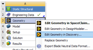
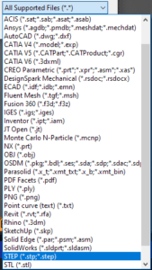
The options to create a crack in Ansys simulation software generally fall in two categories: either a) use a CAD surface that represents the crack, that overlaps with the structure or b) use the auto-generation tool in Ansys to add a crack at the mesh level.
The former works well in all scenarios but is very useful when the crack is not a simple analytical shape, i.e., a penny-shaped crack. The latter is great for those simple, penny-shaped cracks, where the engineer can input two radii to define the shape, input where the crack is located, and they’re done.
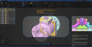
Here’s an example; take this simplified cast bearing/shaft support. The machinist finds a crack when machining the bearing support housing (outlined in the blue box). Perhaps this is caused by an incorrect casting process.
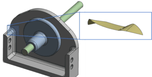
Representative CAD Model, Crack Surface on Right
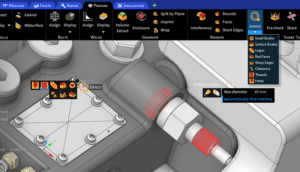
When magnafluxed or cut open, the crack is not a simple shape. This is perhaps an extreme example, but it gets the point across. With a few inputs and clicks, Ansys overlaps the crack surface with the solid CAD, splits the mesh where these intersect, buffers the elements from the new crack mesh into the existing base mesh, and voila! The finite element model crack is ready to analyze.

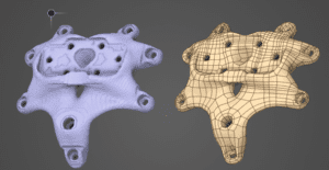
Representative Finite Element Mesh of Structure with Crack Inserted: Back View on Left, Top View on Right (with red line indicating part boundary)
What About Crack Growth?
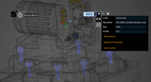
Ansys requires no special treatment of the crack to determine the relevant fracture parameters when evaluating a crack for simple comparison to material fracture toughness. The simplicity of the Ansys workflow mirrors the simplicity of what the engineer is after, i.e., a single value for Stress Intensity Factor. Using the methods described previously, engineers can model a crack and then mesh the structure with hexahedra, tetrahedra, or a mix of element shapes and get results for Stress Intensity Factor.
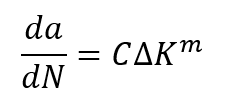
For fatigue cracks, the requirements are greater. Engineers must provide the crack growth equation constants, i.e., the Paris constants C and m, then Ansys will do the rest. Ansys’ technology for general, 3D crack growth is quite extraordinary. This technology is referred to as SMART – Separating, Morphing, and Adaptive Remeshing Technology. To put it simply, automatic remeshing occurs as the crack grows in simulation.

Representative Crack Growth Simulation Showcasing Automated Solution Remeshing
For a nice overview of fracture mechanics in Ansys, you can watch an on-demand webinar on DRD’s website. In the webinar, I provide a brief overview of fracture mechanics and Ansys capabilities in fracture analysis, much like this paper. I also discuss damage tolerant design, material data acquisition, and Ansys CAE simulation of cracks in structures.
Head over to DRD’s website for two on-demand webinars I conducted in October and November, ‘Simulating Crack Propagation Part 1 and 2.’
https://www.drd.com/resources-all/simulating-crack-propagation-part-1-webinar-recording/
https://www.drd.com/resources-all/simulating-crack-propagation-part-2-webinar-recording/
This concludes our 3-part series on fracture mechanics. We have a few other resources engineers can dig into on this topic, including the two on-demand webinars mentioned above. DRD has a fracture mechanics training course that I teach as demand requires, https://www.drd.com/project/ansys-mechanical-fracture-mechanics/. If you are interested in this course, please let us know at support@drd.com.